PyTorch Profiler With TensorBoard

This tutorial demonstrates how to use TensorBoard plugin with PyTorch Profiler to detect performance bottlenecks of the model.

Introduction

PyTorch 1.8 includes an updated profiler API capable of recording the CPU side operations as well as the CUDA kernel launches on the GPU side. The profiler can visualize this information in TensorBoard Plugin and provide analysis of the performance bottlenecks.

In this tutorial, we will use a simple Resnet model to demonstrate how to use TensorBoard plugin to analyze model performance.

Setup

To install torch and torchvision use the following command:

pip install torch torchvision

Steps

1. Prepare the data and model
2. Use profiler to record execution events
3. Run the profiler
4. Use TensorBoard to view results and analyze model performance
5. Improve performance with the help of profiler
6. Analyze performance with other advanced features

1. Prepare the data and model

First, import all necessary libraries:

import torch
import torch.nn
import torch.optim
import torch.profiler
import torch.utils.data
import torchvision.datasets
import torchvision.models
import torchvision.transforms as T

Then prepare the input data. For this tutorial, we use the CIFAR10 dataset. Transform it to the desired format and use DataLoader to load each batch.

transform = T.Compose(
    [T.Resize(224),
     T.ToTensor(),
     T.Normalize((0.5, 0.5, 0.5), (0.5, 0.5, 0.5))])
train_set = torchvision.datasets.CIFAR10(root='./data', train=True, download=True, transform=transform)
train_loader = torch.utils.data.DataLoader(train_set, batch_size=32, shuffle=True)

Next, create Resnet model, loss function, and optimizer objects. To run on GPU, move model and loss to GPU device.

device = torch.device("cuda:0")
model = torchvision.models.resnet18(pretrained=True).cuda(device)
criterion = torch.nn.CrossEntropyLoss().cuda(device)
optimizer = torch.optim.SGD(model.parameters(), lr=0.001, momentum=0.9)
model.train()

Define the training step for each batch of input data.

def train(data):
    inputs, labels = data[0].to(device=device), data[1].to(device=device)
    outputs = model(inputs)
    loss = criterion(outputs, labels)
    optimizer.zero_grad()
    loss.backward()
    optimizer.step()

2. Use profiler to record execution events

The profiler is enabled through the context manager and accepts several parameters, some of the most useful are:

• schedule - callable that takes step (int) as a single parameter and returns the profiler action to perform at each step.

  In this example with wait=1, warmup=1, active=3, repeat=2, profiler will skip the first step/iteration, start warming up on the second, record the following three iterations, after which the trace will become available and on_trace_ready (when set) is called. In total, the cycle repeats twice. Each cycle is called a “span” in TensorBoard plugin.

  During wait steps, the profiler is disabled. During warmup steps, the profiler starts tracing but the results are discarded. This is for reducing the profiling overhead. The overhead at the beginning of profiling is high and easy to bring skew to the profiling result. During active steps, the profiler works and records events.

• on_trace_ready - callable that is called at the end of each cycle; In this example we use torch.profiler.tensorboard_trace_handler to generate result files for TensorBoard. After profiling, result files will be saved into the ./log/resnet18 directory. Specify this directory as a logdir parameter to analyze profile in TensorBoard.

• record_shapes - whether to record shapes of the operator inputs.

• profile_memory - Track tensor memory allocation/deallocation.

• with_stack - Record source information (file and line number) for the ops. If the TensorBoard is launched in VSCode (reference), clicking a stack frame will navigate to the specific code line.

with torch.profiler.profile(
        schedule=torch.profiler.schedule(wait=1, warmup=1, active=3, repeat=2),
        on_trace_ready=torch.profiler.tensorboard_trace_handler('./log/resnet18'),
        record_shapes=True,
        with_stack=True
) as prof:
    for step, batch_data in enumerate(train_loader):
        if step >= (1 + 1 + 3) * 2:
            break
        train(batch_data)
        prof.step()  # Need to call this at the end of each step to notify profiler of steps' boundary.

3. Run the profiler

Run the above code. The profiling result will be saved under ./log/resnet18 directory.

4. Use TensorBoard to view results and analyze model performance

Install PyTorch Profiler TensorBoard Plugin.

pip install torch_tb_profiler

Launch the TensorBoard.

tensorboard --logdir=./log

Open the TensorBoard profile URL in Google Chrome browser or Microsoft Edge browser.

http://localhost:6006/#pytorch_profiler

You could see Profiler plugin page as shown below.

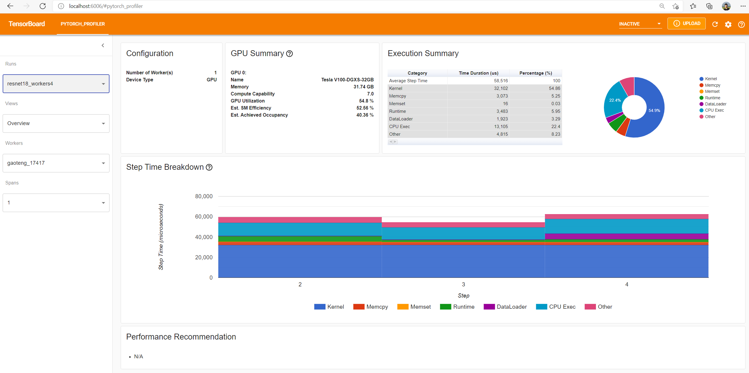
• Overview

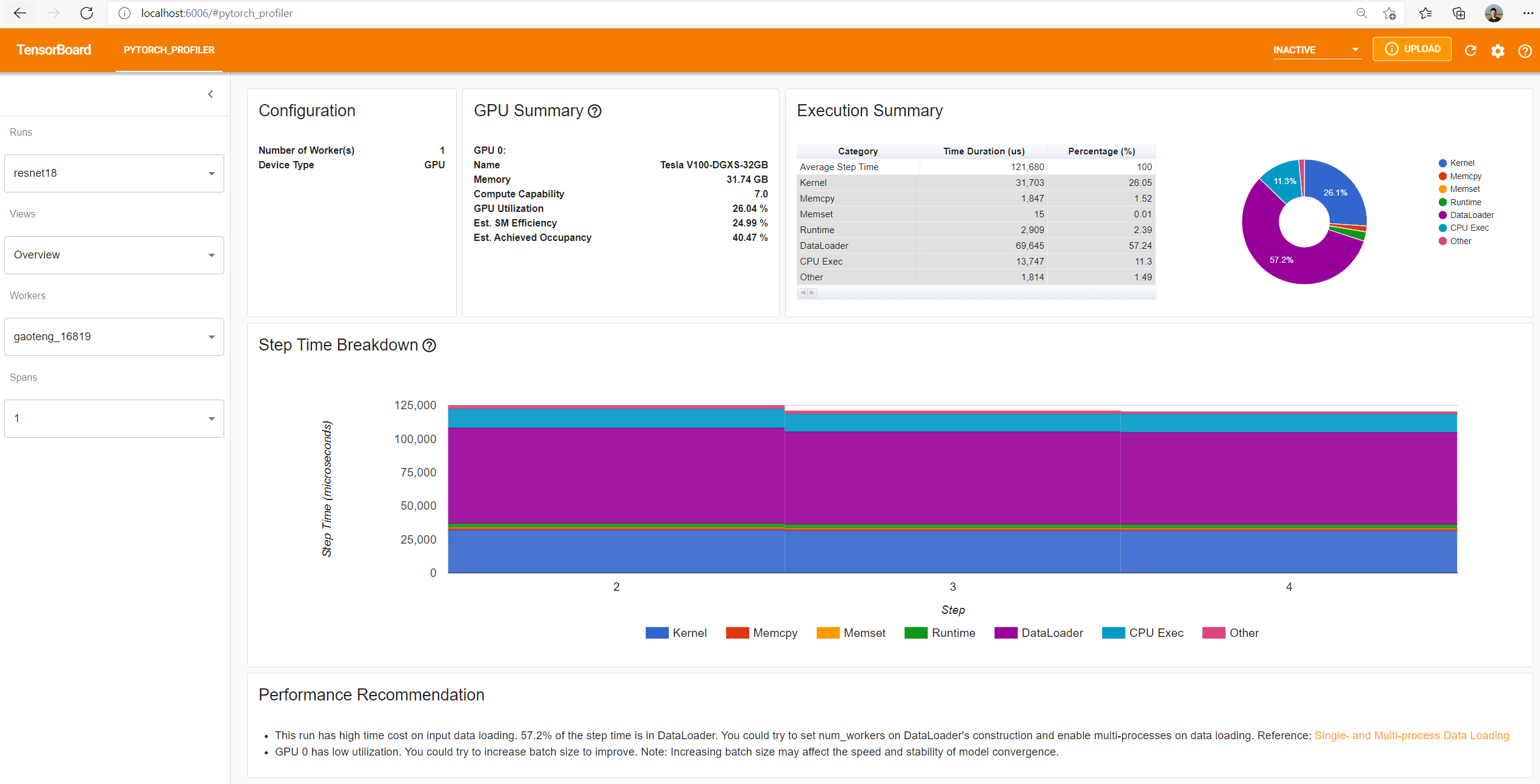
The overview shows a high-level summary of model performance.

The “GPU Summary” panel shows the GPU configuration and the GPU usage. In this example, the GPU Utilization is low. The details of these metrics are here.

The “Step Time Breakdown” shows distribution of time spent in each step over different categories of execution. In this example, you can see the DataLoader overhead is significant.

The bottom “Performance Recommendation” uses the profiling data to automatically highlight likely bottlenecks, and gives you actionable optimization suggestions.

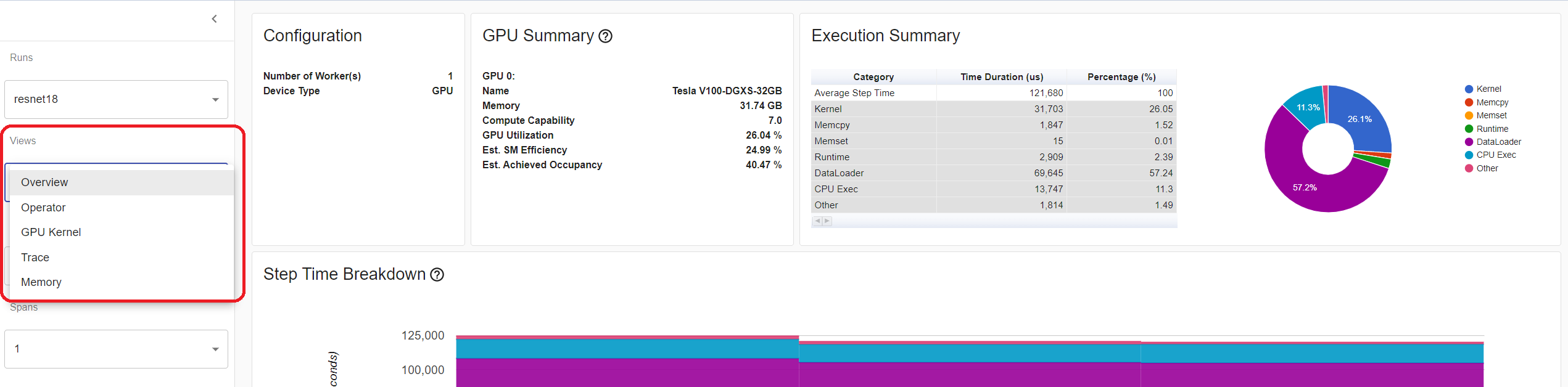
You can change the view page in left “Views” dropdown list.

• Operator view

The operator view displays the performance of every PyTorch operator that is executed either on the host or device.

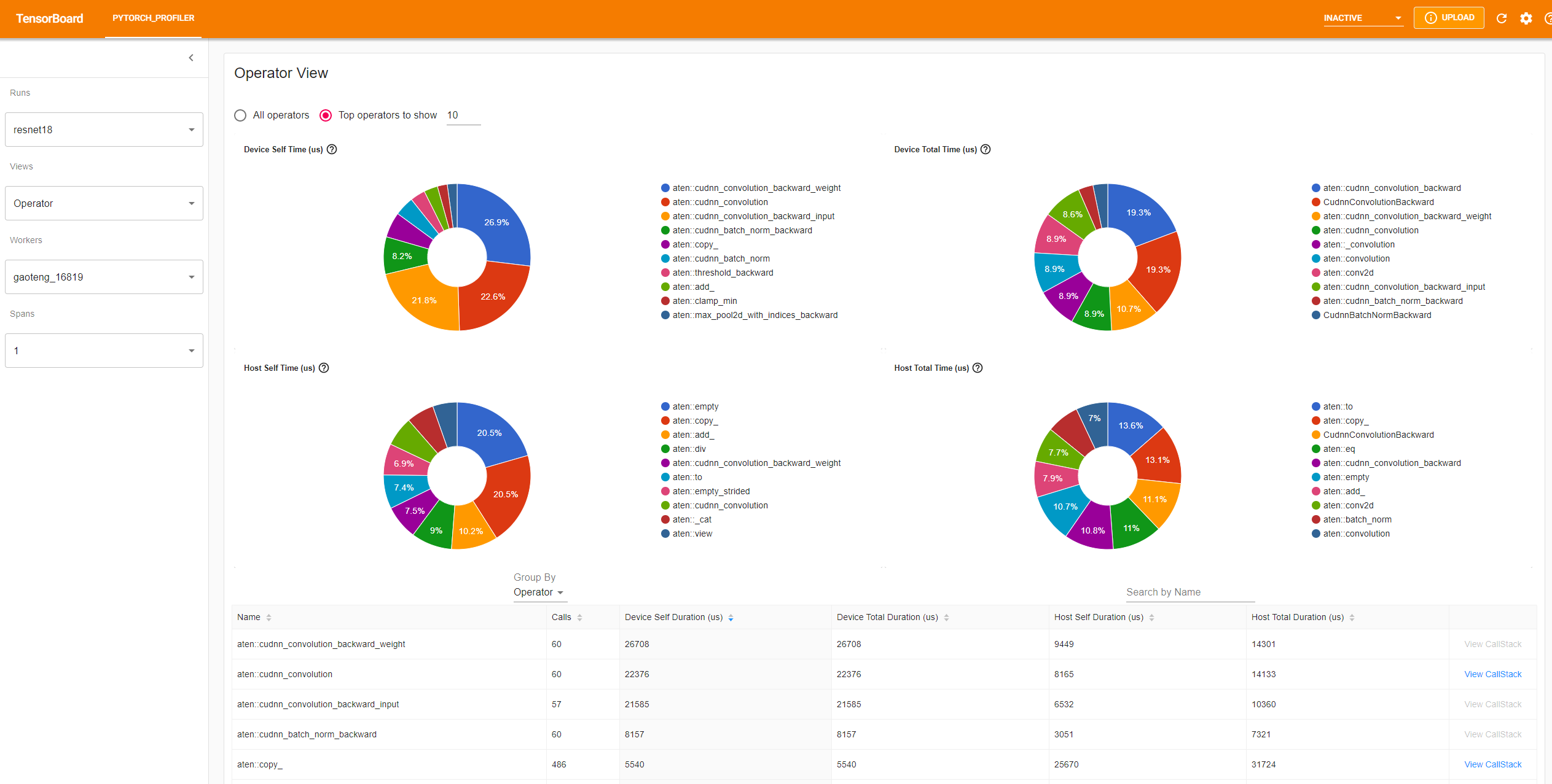
The “Self” duration does not include its child operators’ time. The “Total” duration includes its child operators’ time.

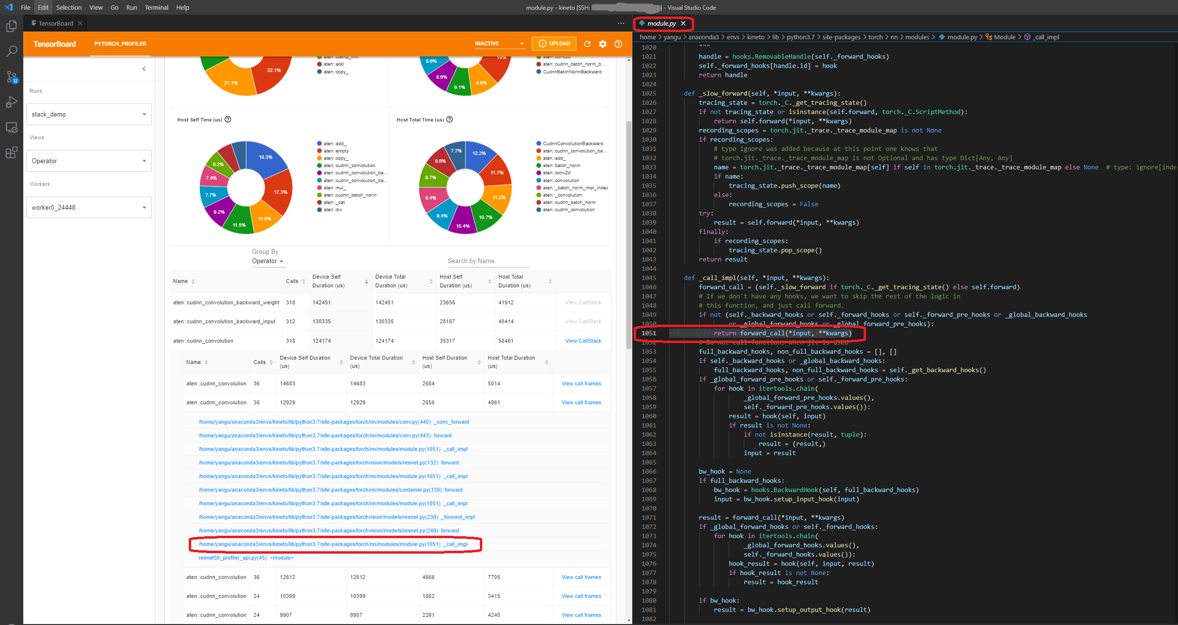
• View call stack

Click the “View Callstack” of an operator, the operators with same name but different call stacks will be shown. Then click a “View Callstack” in this sub-table, the call stack frames will be shown.

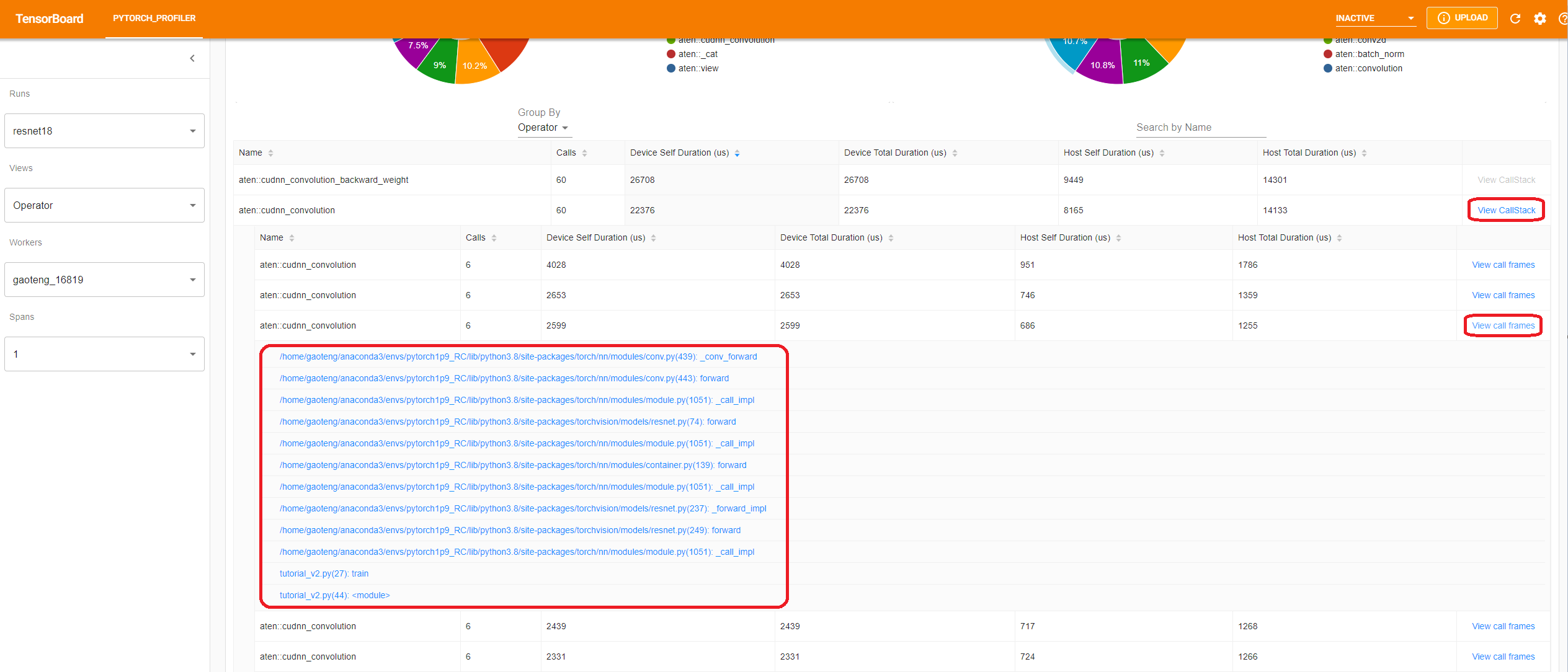
If the TensorBoard is launched inside VSCode (Launch Guide), clicking a call stack frame will navigate to the specific code line.

• Kernel view

The GPU kernel view shows all kernels’ time spent on GPU.

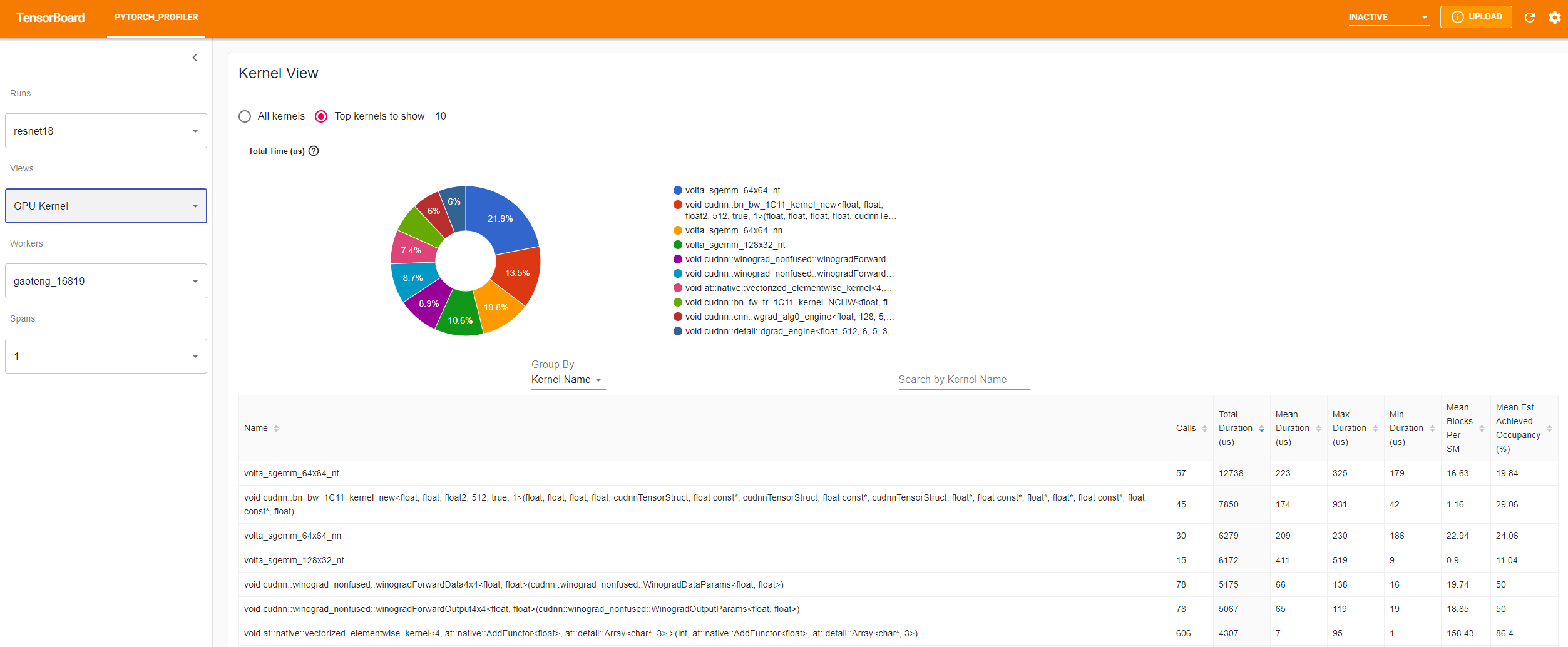
Mean Blocks per SM: Blocks per SM = Blocks of this kernel / SM number of this GPU. If this number is less than 1, it indicates the GPU multiprocessors are not fully utilized. “Mean Blocks per SM” is weighted average of all runs of this kernel name, using each run’s duration as weight.

Mean Est. Achieved Occupancy: Est. Achieved Occupancy is defined in this column’s tooltip. For most cases such as memory bandwidth bounded kernels, the higher the better. “Mean Est. Achieved Occupancy” is weighted average of all runs of this kernel name, using each run’s duration as weight.

• Trace view

The trace view shows timeline of profiled operators and GPU kernels. You can select it to see details as below.

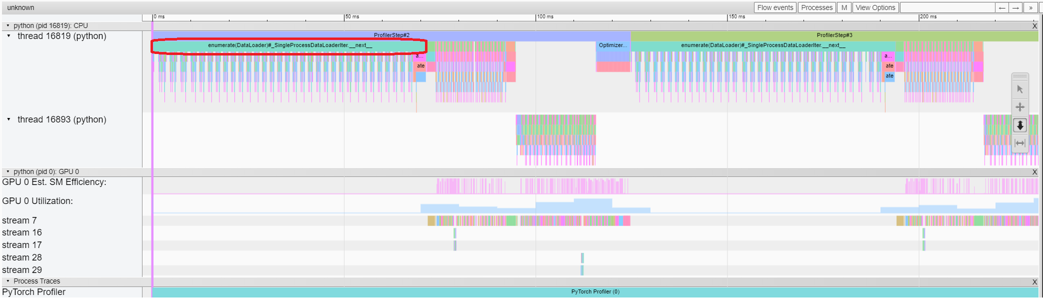
You can move the graph and zoom in/out with the help of right side toolbar. And keyboard can also be used to zoom and move around inside the timeline. The ‘w’ and ‘s’ keys zoom in centered around the mouse, and the ‘a’ and ‘d’ keys move the timeline left and right. You can hit these keys multiple times until you see a readable representation.

In this example, we can see the event prefixed with enumerate(DataLoader) costs a lot of time. And during most of this period, the GPU is idle. Because this function is loading data and transforming data on host side, during which the GPU resource is wasted.

5. Improve performance with the help of profiler

At the bottom of “Overview” page, the suggestion in “Performance Recommendation” hints the bottleneck is DataLoader. The PyTorch DataLoader uses single process by default. User could enable multi-process data loading by setting the parameter num_workers. Here is more details.

In this example, we follow the “Performance Recommendation” and set num_workers as below, pass a different name such as ./log/resnet18_4workers to tensorboard_trace_handler, and run it again.

train_loader = torch.utils.data.DataLoader(train_set, batch_size=32, shuffle=True, num_workers=4)

Then let’s choose the recently profiled run in left “Runs” dropdown list.

From the above view, we can find the step time is reduced to about 58ms comparing with previous run’s 121ms, and the time reduction of DataLoader mainly contributes.

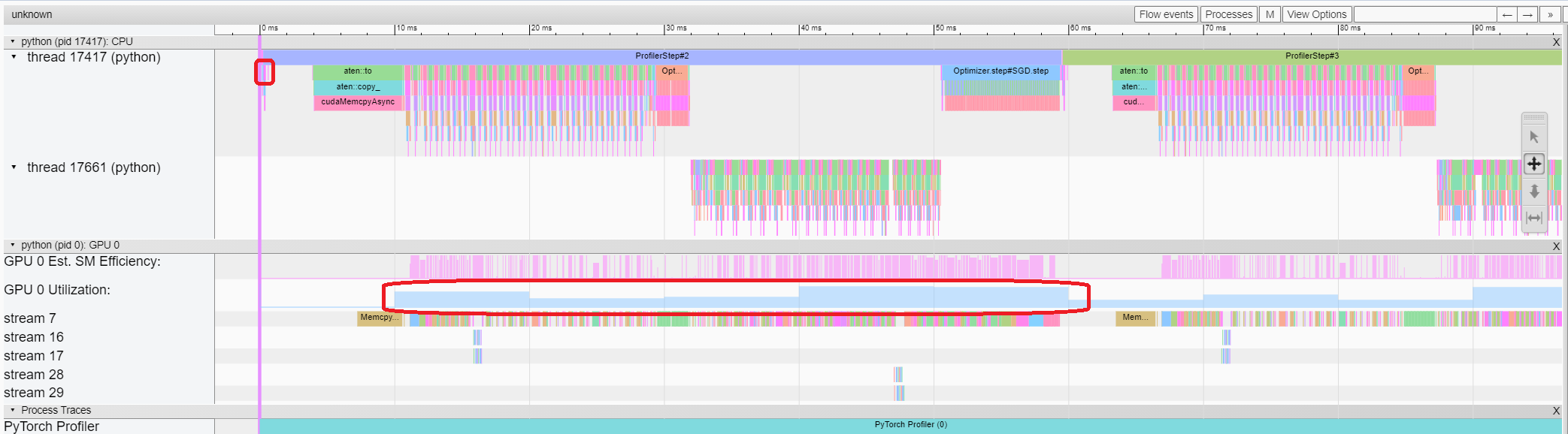
From the above view, we can see that the runtime of enumerate(DataLoader) is reduced, and the GPU utilization is increased.

6. Analyze performance with other advanced features

• Memory view

To profile memory, please add profile_memory=True in arguments of torch.profiler.profile.

Note: Because of the current non-optimized implementation of PyTorch profiler, enabling profile_memory=True will take about several minutes to finish. To save time, you can try our existing examples first by running:

tensorboard --logdir=https://torchtbprofiler.blob.core.windows.net/torchtbprofiler/demo/memory_demo

The profiler records all memory allocation/release events during profiling. For every specific operator, the plugin aggregates all these memory events inside its life span.

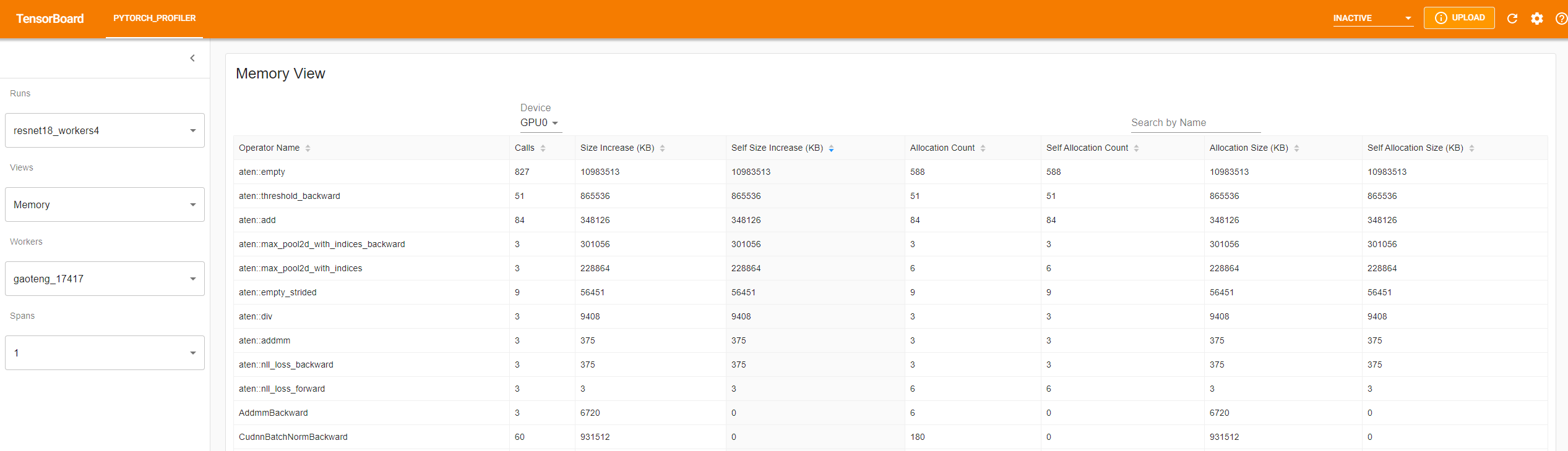
The memory type could be selected in “Device” selection box. For example, “GPU0” means the following table only shows each operator’s memory usage on GPU 0, not including CPU or other GPUs.

The “Size Increase” sums up all allocation bytes and minus all the memory release bytes.

The “Allocation Size” sums up all allocation bytes without considering the memory release.

• Distributed view

The plugin now supports distributed view on profiling DDP with NCCL as backend.

You can try it by using existing example on Azure:

tensorboard --logdir=https://torchtbprofiler.blob.core.windows.net/torchtbprofiler/demo/distributed_bert

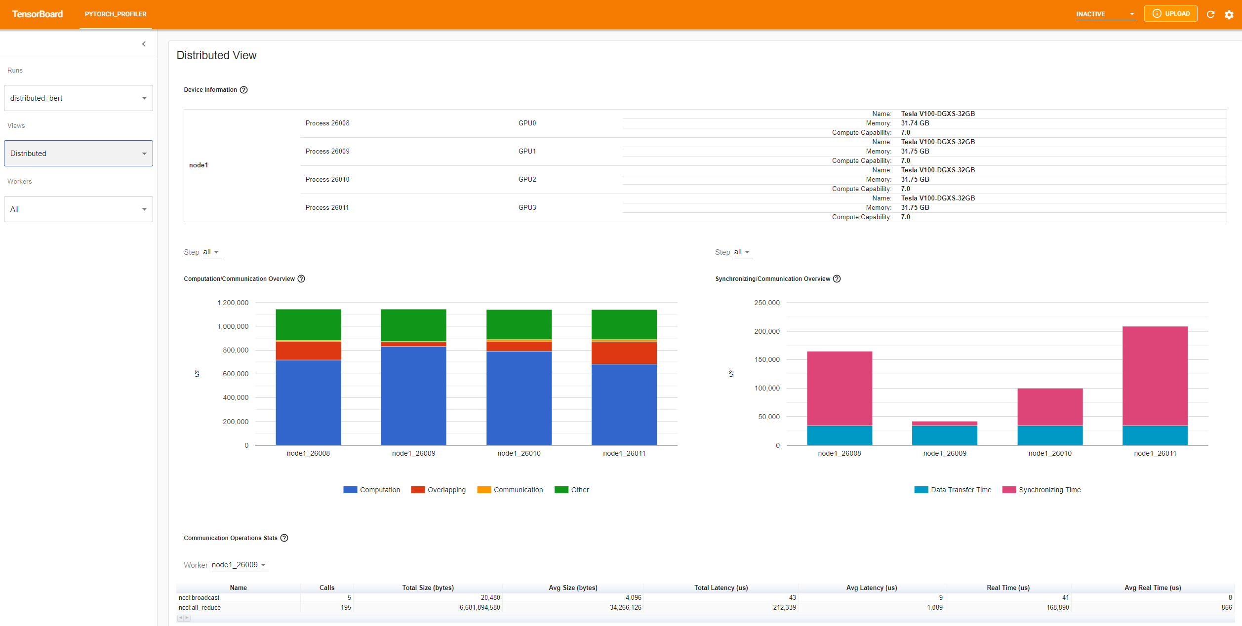
The “Computation/Communication Overview” shows computation/communication ratio and their overlapping degree. From this view, User can figure out load balance issue among workers. For example, if the computation + overlapping time of one worker is much larger than others, there may be a problem of load balance or this worker may be a straggler.

The “Synchronizing/Communication Overview” shows the efficiency of communication. “Data Transfer Time” is the time for actual data exchanging. “Synchronizing Time” is the time for waiting and synchronizing with other workers.

If one worker’s “Synchronizing Time” is much shorter than that of other workers’, this worker may be a straggler which may have more computation workload than other workers’.

The “Communication Operations Stats” summarizes the detailed statistics of all communication ops in each worker.

Learn More

Take a look at the following documents to continue your learning, and feel free to open an issue here.

• Pytorch TensorBoard Profiler github
• torch.profiler API